Regional Analysis with T1 and DWI Data
This notebook demonstrates how to combine structural (T1) and diffusion (DWI) MRI
using kwneuro to perform brain region-level microstructure analysis. We use a
dataset from openneuro, which includes a T1 and a single-shell DWI
acquisition.
Pipeline overview
Download example data
Load DWI and T1 data
T1 bias correction
T1 brain extraction and tissue segmentation (Atropos vs Deep Atropos)
Cortical parcellation (DKT atlas via ANTsPyNet)
DWI preprocessing: denoising, brain extraction, and DTI estimation
Register DWI to T1 space (rigid body)
Warp parcellation labels into DWI space
0. Download example data
We download one subject from the MPI-Leipzig Mind-Brain-Body dataset (OpenNeuro ds000221). This dataset contains 64-direction single-shell DWI data (b ~ 1000 s/mm²) and a T1-weighted structural image.
The data is downloaded automatically on first run (~100 MB).
from pathlib import Path

import openneuro as on

DATA_DIR = Path("example_data/ds000221")
SUBJECT, SESSION = "sub-010002", "ses-01"

t1_path = DATA_DIR / SUBJECT / SESSION / "anat" / f"{SUBJECT}_{SESSION}_acq-mp2rage_T1w.nii.gz"
dwi_dir = DATA_DIR / SUBJECT / SESSION / "dwi"

if not t1_path.exists() or not dwi_dir.exists() or not list(dwi_dir.glob("*_dwi.nii.gz")):
    DATA_DIR.mkdir(parents=True, exist_ok=True)
    on.download(
        dataset="ds000221",
        target_dir=str(DATA_DIR),
        include=[
            "dataset_description.json",
            f"{SUBJECT}/{SESSION}/anat/*T1w*",
            f"{SUBJECT}/{SESSION}/dwi/*",
        ],
    )

dwi_nii = next(dwi_dir.glob("*_dwi.nii.gz"))
basename = dwi_nii.name.removesuffix(".nii.gz")

print(f"T1 path:      {t1_path}")
print(f"DWI dir:      {dwi_dir}")
print(f"DWI basename: {basename}")
1. Load T1 data
The T1-weighted structural image provides the anatomical reference for tissue segmentation, cortical parcellation, and DWI co-registration.
import matplotlib
import matplotlib.pyplot as plt
import numpy as np

from kwneuro.dwi import Dwi
from kwneuro.io import FslBvalResource, FslBvecResource, NiftiVolumeResource
from kwneuro.reg import register_dwi_to_structural
from kwneuro.structural import StructuralImage

structural = StructuralImage(NiftiVolumeResource(t1_path)).load()

if SUBSAMPLE:
    from kwneuro.util import subsample_volume

    structural = StructuralImage(subsample_volume(structural.volume, SUBSAMPLE_FACTOR))
    print(f"Subsampled T1 by factor {SUBSAMPLE_FACTOR}")

struct_image = structural.volume.get_array()
t1_mid = struct_image.shape[2] // 2
t1_slice = 170

print(f"T1 shape: {struct_image.shape}")
T1 shape: (176, 240, 256)
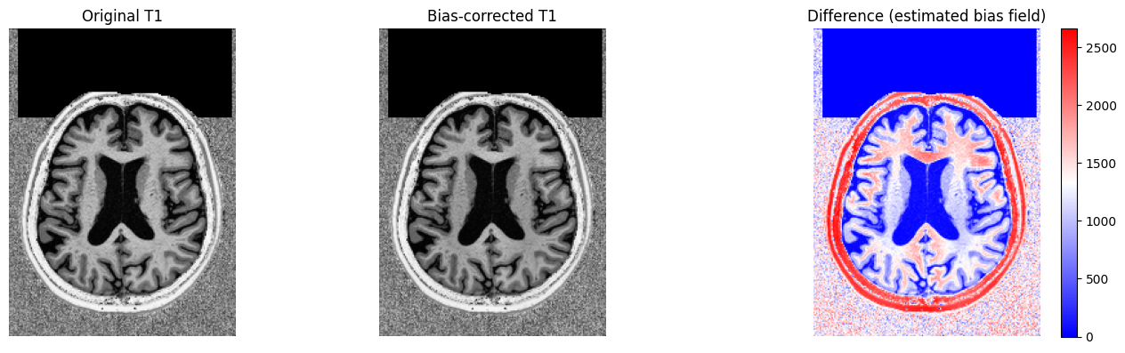
2. T1 bias correction
RF field inhomogeneities create smooth intensity gradients across the T1 that
can bias tissue segmentation and parcellation. correct_bias() applies ANTsPy’s
N4 bias field correction before downstream structural processing.
structural_bc = structural.correct_bias()
t1_bc = structural_bc.volume.get_array()

fig, axes = plt.subplots(1, 3, figsize=(14, 4))
axes[0].imshow(struct_image[:, :, t1_slice].T, cmap="gray", origin="lower")
axes[0].set_title("Original T1")
axes[1].imshow(t1_bc[:, :, t1_slice].T, cmap="gray", origin="lower")
axes[1].set_title("Bias-corrected T1")
diff = t1_bc[:,:, t1_slice] - struct_image[:, :, t1_slice]
im = axes[2].imshow(diff.T, cmap="bwr", origin="lower")
axes[2].set_title("Difference (estimated bias field)")
plt.colorbar(im, ax=axes[2], fraction=0.046)
for ax in axes:
    ax.axis("off")
plt.tight_layout()
plt.show()
Load DWI data
A Dwi object bundles the 4D volume, b-values, and b-vectors.
dwi = Dwi(
    NiftiVolumeResource(dwi_dir / f"{basename}.nii.gz"),
    FslBvalResource(dwi_dir / f"{basename}.bval"),
    FslBvecResource(dwi_dir / f"{basename}.bvec"),
).load()

vol = dwi.volume.get_array()
bvals = dwi.bval.get()
dwi_mid = vol.shape[2] // 2

print(f"DWI shape: {vol.shape}")
print(f"Unique b-values: {np.unique(np.round(bvals, -2))}")
DWI shape: (128, 128, 88, 67)
Unique b-values: [   0. 1000.]
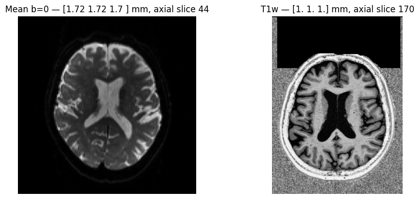
The two images have very different resolutions and field-of-view sizes — the DWI covers only a portion of the brain while the T1 spans the full volume. This is typical of real acquisitions and is exactly what the registration step handles.
t1_affine = structural_bc.volume.get_affine()
dwi_affine = dwi.volume.get_affine()

t1_vox_size = np.linalg.norm(t1_affine[:3, :3], axis=0).round(2)
dwi_vox_size = np.linalg.norm(dwi_affine[:3, :3], axis=0).round(2)

print(f"T1 voxel size:  {t1_vox_size} mm")
print(f"DWI voxel size: {dwi_vox_size} mm")

mean_b0 = dwi.compute_mean_b0()
mean_b0_arr = mean_b0.get_array()

fig, axes = plt.subplots(1, 2, figsize=(10, 4))
axes[0].imshow(mean_b0_arr[:, :, dwi_mid].T, cmap="gray", origin="lower")
axes[0].set_title(f"Mean b=0 — {dwi_vox_size} mm, axial slice {dwi_mid}")
axes[1].imshow(struct_image[:, :, t1_slice].T, cmap="gray", origin="lower")
axes[1].set_title(f"T1w — {t1_vox_size} mm, axial slice {t1_slice}")
for ax in axes:
    ax.axis("off")
plt.tight_layout()
plt.show()
T1 voxel size:  [1. 1. 1.] mm
DWI voxel size: [1.72 1.72 1.7 ] mm
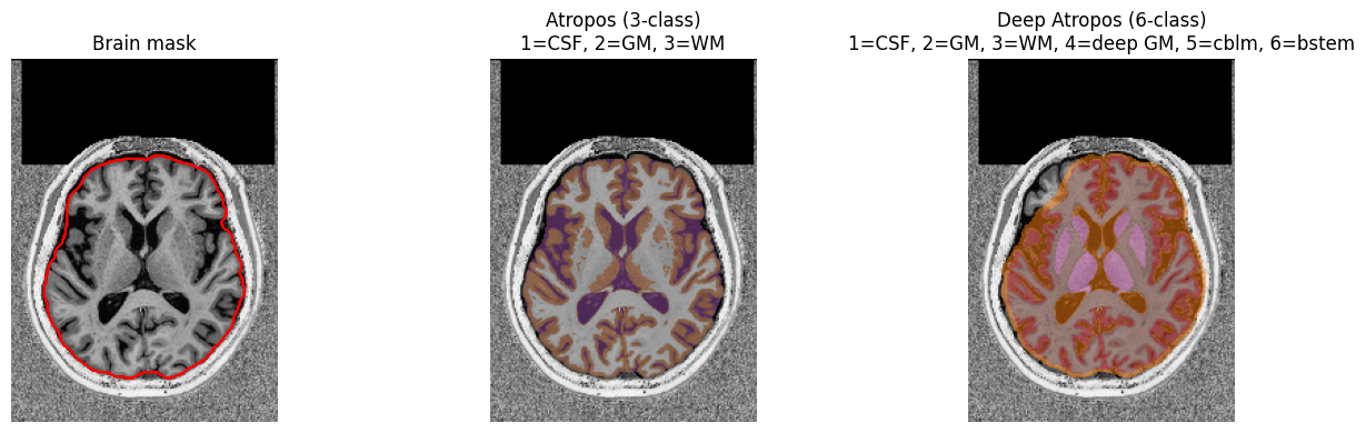
3. Brain extraction and tissue segmentation
We extract a brain mask from the bias-corrected T1 using HD-BET, then compare two tissue segmentation methods:
Atropos (default): classical ANTsPy k-means, 3 classes — CSF (1), GM (2), WM (3).
Deep Atropos: deep-learning segmentation via ANTsPyNet, 6 classes — CSF (1), GM (2), WM (3), deep GM (4), cerebellum (5), brainstem (6). Requires
pip install kwneuro[antspynet].
t1_mask = structural_bc.extract_brain()
segmentation = structural_bc.segment_tissues(mask=t1_mask)
segmentation_deep = structural_bc.segment_tissues(method="deep_atropos")

seg_arr = segmentation.get_array()
seg_deep_arr = segmentation_deep.get_array()
t1_mask_arr = t1_mask.get_array()

t1_slc = t1_bc[:, :, t1_slice].T

fig, axes = plt.subplots(1, 3, figsize=(14, 4))

axes[0].imshow(t1_slc, cmap="gray", origin="lower")
axes[0].contour(t1_mask_arr[:, :, t1_slice].T, colors="red", linewidths=0.8)
axes[0].set_title("Brain mask")

axes[1].imshow(t1_slc, cmap="gray", origin="lower")
axes[1].imshow(
    np.ma.masked_equal(seg_arr[:, :, t1_slice].T, 0),
    cmap=matplotlib.colormaps.get_cmap("Set1").resampled(4),
    origin="lower",
    vmin=0,
    vmax=3,
    alpha=0.5,
)
axes[1].set_title("Atropos (3-class)\n1=CSF, 2=GM, 3=WM")

axes[2].imshow(t1_slc, cmap="gray", origin="lower")
axes[2].imshow(
    np.ma.masked_equal(seg_deep_arr[:, :, t1_slice].T, 0),
    cmap=matplotlib.colormaps.get_cmap("tab10").resampled(7),
    origin="lower",
    vmin=0,
    vmax=6,
    alpha=0.5,
)
axes[2].set_title("Deep Atropos (6-class)\n1=CSF, 2=GM, 3=WM, 4=deep GM, 5=cblm, 6=bstem")

for ax in axes:
    ax.axis("off")
plt.tight_layout()
plt.show()
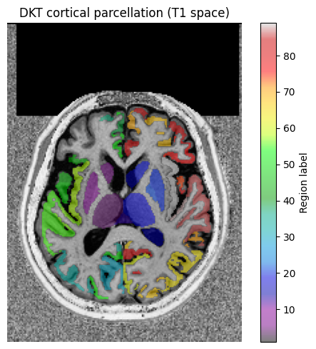
4. Cortical parcellation (DKT atlas)
parcellate(method="dkt") applies the Desikan-Killiany-Tourville (DKT) cortical
labeling via ANTsPyNet. A deep learning model assigns each cortical voxel to one of
approximately 84 regions directly from the T1 image.
Note: This step requires
pip install kwneuro[antspynet]and sufficient RAM (~8 GB free) to run the deep-learning model on a full-resolution T1.
parcellation = structural_bc.parcellate(method="dkt")
parc_arr = parcellation.get_array()

# Remap labels to sequential 1-N
labels_present = np.unique(parc_arr)
labels_present = labels_present[labels_present != 0]
label_to_idx = {label: idx + 1 for idx, label in enumerate(labels_present)}
parc_remapped = np.vectorize(label_to_idx.get)(parc_arr, 0)  # 0 stays as background

print(f"Parcellation shape: {parc_arr.shape}")
print(f"Distinct labels (including background 0): {len(labels_present)}")

fig, ax = plt.subplots(figsize=(6, 5))
ax.imshow(t1_bc[:, :, t1_slice].T, cmap="gray", origin="lower")
im = ax.imshow(
    np.ma.masked_equal(parc_remapped[:, :, t1_slice].T, 0),
    cmap="nipy_spectral",
    origin="lower",
    alpha=0.5,
    vmin=1,
    vmax=len(labels_present),
)
ax.set_title("DKT cortical parcellation (T1 space)")
ax.axis("off")
plt.colorbar(im, ax=ax, fraction=0.046, label="Region label")
plt.tight_layout()
plt.show()
Parcellation shape: (176, 240, 256)
Distinct labels (including background 0): 89
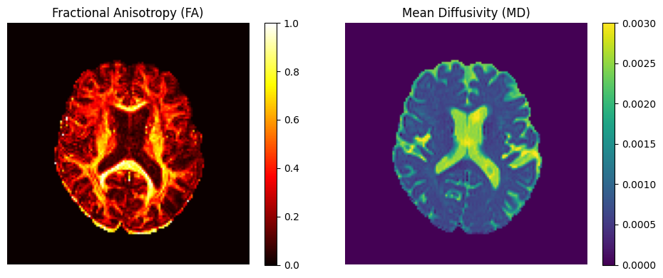
5. DWI preprocessing
Three steps prepare the DWI for registration and DTI estimation: Patch2Self denoising, HD-BET brain extraction, and DIPY TensorModel fitting.
dwi_denoised = dwi.denoise()
dwi_mask = dwi_denoised.extract_brain()
dti = dwi_denoised.estimate_dti(mask=dwi_mask)
fa_vol, md_vol = dti.get_fa_md()
fa = fa_vol.get_array()
md = md_vol.get_array()

mean_b0_denoised = dwi_denoised.compute_mean_b0()
mean_b0_denoised_arr = mean_b0_denoised.get_array()

fig, axes = plt.subplots(1, 2, figsize=(10, 4))
im1 = axes[0].imshow(fa[:, :, dwi_mid].T, cmap="hot", origin="lower", vmin=0, vmax=1)
axes[0].set_title("Fractional Anisotropy (FA)")
plt.colorbar(im1, ax=axes[0], fraction=0.046)
im2 = axes[1].imshow(
    md[:, :, dwi_mid].T, cmap="viridis", origin="lower", vmin=0, vmax=3e-3
)
axes[1].set_title("Mean Diffusivity (MD)")
plt.colorbar(im2, ax=axes[1], fraction=0.046)
for ax in axes:
    ax.axis("off")
plt.tight_layout()
plt.show()
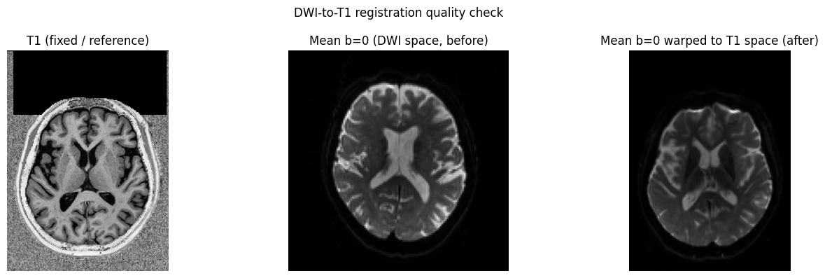
6. Register DWI to T1 space (rigid body)
A rigid-body transform aligns the mean b=0 image to the T1. A rigid transform is appropriate here because the DWI and T1 were acquired in the same session — we only need to correct for minor inter-sequence head motion.
transform = register_dwi_to_structural(
    dwi=dwi_denoised,
    structural=structural_bc,
    type_of_transform="SyN",
    dwi_mask=dwi_mask,
    structural_mask=t1_mask,
)
# Verify registration quality: warp the mean b=0 forward into T1 space
registered_b0 = transform.apply(
    fixed=structural_bc.volume,
    moving=mean_b0_denoised,
)
reg_arr = registered_b0.get_array()

fig, axes = plt.subplots(1, 3, figsize=(14, 4))
axes[0].imshow(t1_bc[:, :, t1_slice].T, cmap="gray", origin="lower")
axes[0].set_title("T1 (fixed / reference)")
axes[1].imshow(mean_b0_denoised_arr[:, :, dwi_mid].T, cmap="gray", origin="lower")
axes[1].set_title("Mean b=0 (DWI space, before)")
axes[2].imshow(reg_arr[:, :, t1_slice].T, cmap="gray", origin="lower")
axes[2].set_title("Mean b=0 warped to T1 space (after)")
for ax in axes:
    ax.axis("off")
plt.suptitle("DWI-to-T1 registration quality check")
plt.tight_layout()
plt.show()
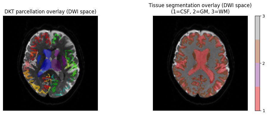
7. Warp labels into DWI space
To analyse DTI values per brain region we need the parcel labels in the same space as the DTI maps. We apply the inverse of the DWI→T1 transform to warp both the DKT parcellation and the Atropos tissue segmentation into DWI space.
interpolation="genericLabel" uses nearest-neighbour resampling, which preserves
integer label values without blending across region boundaries.
parcellation_dwi = transform.apply(
    fixed=mean_b0_denoised,
    moving=parcellation,
    invert=True,
    interpolation="genericLabel",
)
parc_dwi_arr = parcellation_dwi.get_array()

labels_present = np.unique(parc_dwi_arr)
labels_present = labels_present[labels_present != 0]
label_to_idx = {label: idx + 1 for idx, label in enumerate(labels_present)}
parc_dwi_remapped = np.vectorize(label_to_idx.get)(parc_dwi_arr, 0)  # 0 stays as background

segmentation_dwi = transform.apply(
    fixed=mean_b0_denoised,
    moving=segmentation,
    invert=True,
    interpolation="genericLabel",
)
seg_dwi_arr = segmentation_dwi.get_array()

fig, axes = plt.subplots(1, 2, figsize=(10, 4))

axes[0].imshow(mean_b0_denoised_arr[:, :, dwi_mid].T, cmap="gray", origin="lower")
axes[0].imshow(
    np.ma.masked_equal(parc_dwi_remapped[:, :, 40], 0).T,
    cmap="nipy_spectral",
    origin="lower",
    alpha=0.55,
)
axes[0].set_title("DKT parcellation overlay (DWI space)")
axes[0].axis("off")

seg_cmap = matplotlib.colormaps.get_cmap("Set1").resampled(4)
axes[1].imshow(mean_b0_denoised_arr[:, :, dwi_mid].T, cmap="gray", origin="lower")
im = axes[1].imshow(
    np.ma.masked_equal(seg_dwi_arr[:, :, dwi_mid], 0).T,
    cmap=seg_cmap,
    origin="lower",
    vmin=1,
    vmax=3,
    alpha=0.5,
)
axes[1].set_title("Tissue segmentation overlay (DWI space)\n(1=CSF, 2=GM, 3=WM)")
axes[1].axis("off")
plt.colorbar(im, ax=axes[1], fraction=0.046, ticks=[1, 2, 3])

plt.tight_layout()
plt.show()