Single-Subject Microstructure Pipeline
This notebook demonstrates the main capabilities of the kwneuro package
for extracting brain microstructure parameters from diffusion MRI data.
Download example data
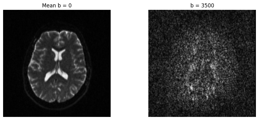
We use the Sherbrooke 3-shell HARDI dataset from DIPY, which provides multi-shell diffusion data (b = 0, 1000, 2000, 3500 s/mm²) with 193 gradient directions. Multi-shell data is required for NODDI estimation.
The data is downloaded automatically on first run (~50 MB).
from dipy.data import fetch_sherbrooke_3shell

# Download the dataset if not already present
files, data_dir = fetch_sherbrooke_3shell()
basename = "HARDI193"

print(f"Data directory: {data_dir}")
print(f"Files: {list(files.keys())}")
Load DWI data
A Dwi object bundles three resources: the 4D volume, b-values, and
b-vectors. Resources are loaded lazily — nothing is read from disk until
you call .load().
from pathlib import Path

import matplotlib.pyplot as plt
import numpy as np

from kwneuro.dwi import Dwi
from kwneuro.io import FslBvalResource, FslBvecResource, NiftiVolumeResource

data_dir = Path(data_dir)

dwi = Dwi(
    NiftiVolumeResource(data_dir / f"{basename}.nii.gz"),
    FslBvalResource(data_dir / f"{basename}.bval"),
    FslBvecResource(data_dir / f"{basename}.bvec"),
).load()

if SUBSAMPLE:
    from kwneuro.dwi import subsample_dwi

    dwi = subsample_dwi(dwi, SUBSAMPLE_FACTOR)
    print(f"Subsampled by factor {SUBSAMPLE_FACTOR}")

vol = dwi.volume.get_array()
bvals = dwi.bval.get()
print(f"Volume shape: {vol.shape}")
print(f"Unique b-values: {np.unique(np.round(bvals, -2))}")
Volume shape: (128, 128, 60, 193)
Unique b-values: [   0. 1000. 2000. 3500.]
Quick look at the mean b=0 image and a diffusion-weighted image side by side.
compute_mean_b0() averages all b=0 volumes, which is also used internally
by brain extraction.
mean_b0 = dwi.compute_mean_b0()
mean_b0_arr = mean_b0.get_array()
mid_slice = vol.shape[2] // 2
dwi_large_bval_idx = np.argmax(bvals)
fig, axes = plt.subplots(1, 2, figsize=(10, 4))
axes[0].imshow(mean_b0_arr[:, :, mid_slice].T, cmap="gray", origin="lower")
axes[0].set_title("Mean b = 0")
axes[1].imshow(vol[:, :, mid_slice, dwi_large_bval_idx].T, cmap="gray", origin="lower")
axes[1].set_title(f"b = {bvals[dwi_large_bval_idx]:.0f}")
for ax in axes:
    ax.axis("off")
plt.tight_layout()
plt.show()
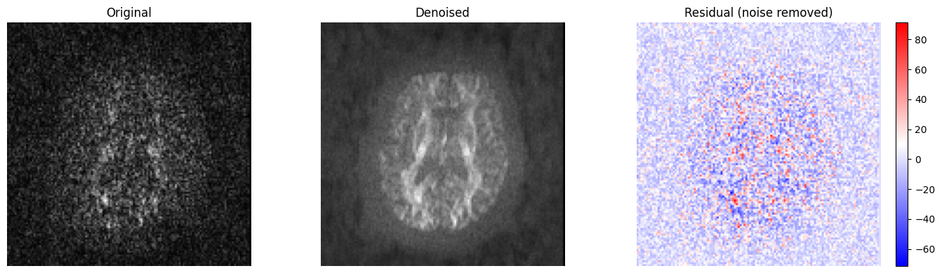
Denoising
Dwi.denoise() applies DIPY’s Patch2Self algorithm. It returns a new Dwi
with the denoised volume (b-values and b-vectors are carried forward
unchanged).
dwi_denoised = dwi.denoise()
orig = vol[:, :, mid_slice, dwi_large_bval_idx]
denoised_large_bval = dwi_denoised.volume.get_array()[:, :, mid_slice, dwi_large_bval_idx]

fig, axes = plt.subplots(1, 3, figsize=(14, 4))
axes[0].imshow(orig.T, cmap="gray", origin="lower")
axes[0].set_title("Original")
axes[1].imshow(denoised_large_bval.T, cmap="gray", origin="lower")
axes[1].set_title("Denoised")
im = axes[2].imshow((orig - denoised_large_bval).T, cmap="bwr", origin="lower")
axes[2].set_title("Residual (noise removed)")
plt.colorbar(im, ax=axes[2], fraction=0.046)
for ax in axes:
    ax.axis("off")
plt.tight_layout()
plt.show()
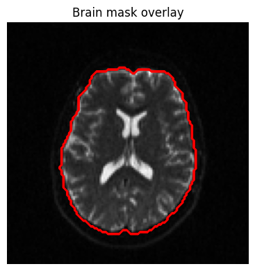
Brain extraction
extract_brain() uses HD-BET to produce a binary brain mask from the mean
b=0 image. The mask is returned as a VolumeResource.
mask = dwi_denoised.extract_brain()
mask_arr = mask.get_array()
denoised = dwi_denoised.compute_mean_b0().get_array()[:, :, mid_slice]
print(f"Mask shape: {mask_arr.shape}, voxels in brain: {mask_arr.sum()}")

fig, ax = plt.subplots(figsize=(5, 4))
ax.imshow(denoised.T, cmap="gray", origin="lower")
ax.contour(mask_arr[:, :, mid_slice].T, colors="red", linewidths=0.8)
ax.set_title("Brain mask overlay")
ax.axis("off")
plt.tight_layout()
plt.show()
Mask shape: (128, 128, 60), voxels in brain: 174687.0
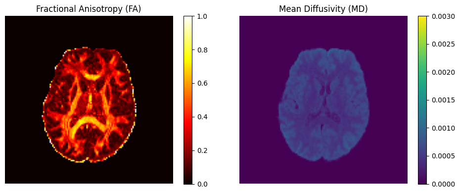
DTI estimation
estimate_dti() fits a diffusion tensor at each voxel using DIPY’s
TensorModel. The resulting Dti object gives access to:
FA (fractional anisotropy) — degree of diffusion directionality
MD (mean diffusivity) — average diffusion rate
Eigenvalues / eigenvectors — full tensor decomposition
dti = dwi_denoised.estimate_dti(mask=mask)
fa_vol, md_vol = dti.get_fa_md()
fa = fa_vol.get_array()
md = md_vol.get_array()

fig, axes = plt.subplots(1, 2, figsize=(10, 4))
im0 = axes[0].imshow(fa[:, :, mid_slice].T, cmap="hot", origin="lower", vmin=0, vmax=1)
axes[0].set_title("Fractional Anisotropy (FA)")
plt.colorbar(im0, ax=axes[0], fraction=0.046)
im1 = axes[1].imshow(
    md[:, :, mid_slice].T, cmap="viridis", origin="lower", vmin=0, vmax=3e-3
)
axes[1].set_title("Mean Diffusivity (MD)")
plt.colorbar(im1, ax=axes[1], fraction=0.046)
for ax in axes:
    ax.axis("off")
plt.tight_layout()
plt.show()
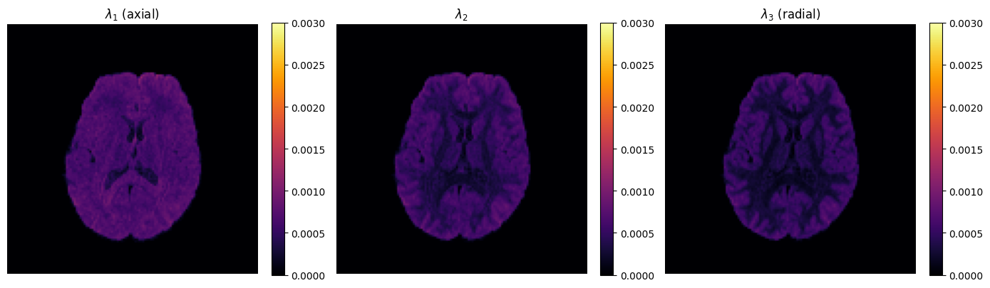
Eigenvalue decomposition
The eigenvalues ($\lambda_1 \ge \lambda_2 \ge \lambda_3$) reveal the shape of diffusion at each voxel.
evals_vol, evecs_vol = dti.get_eig()
evals = evals_vol.get_array()  # shape (x, y, z, 3)

fig, axes = plt.subplots(1, 3, figsize=(14, 4))
for i, (ax, label) in enumerate(
    zip(axes, [r"$\lambda_1$ (axial)", r"$\lambda_2$", r"$\lambda_3$ (radial)"])
):
    im = ax.imshow(
        evals[:, :, mid_slice, i].T, cmap="inferno", origin="lower", vmin=0, vmax=3e-3
    )
    ax.set_title(label)
    ax.axis("off")
    plt.colorbar(im, ax=ax, fraction=0.046)
plt.tight_layout()
plt.show()
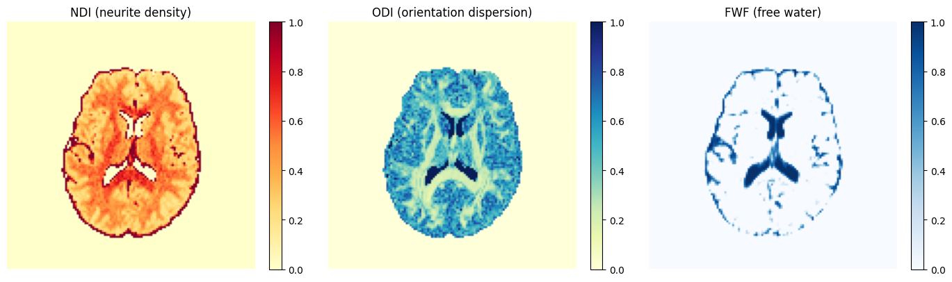
NODDI estimation
estimate_noddi() fits a NODDI model at each voxel using AMICO. The resulting Noddi object
gives access to the following biophysically meaningful parameters:
NDI — neurite density index
ODI — orientation dispersion index
FWF — free water fraction
noddi = dwi_denoised.estimate_noddi(mask=mask) # array shape (x, y, z, 3)
fig, axes = plt.subplots(1, 3, figsize=(14, 4))
for ax, arr, title, cmap in [
    (axes[0], noddi.ndi.get_array()[:, :, mid_slice], "NDI (neurite density)", "YlOrRd"),
    (axes[1], noddi.odi.get_array()[:, :, mid_slice], "ODI (orientation dispersion)", "YlGnBu"),
    (axes[2], noddi.fwf.get_array()[:, :, mid_slice], "FWF (free water)", "Blues"),
]:
    im = ax.imshow(arr.T, cmap=cmap, origin="lower", vmin=0, vmax=1)
    ax.set_title(title)
    ax.axis("off")
    plt.colorbar(im, ax=ax, fraction=0.046)
plt.tight_layout()
plt.show()
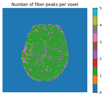
CSD and fiber orientation distributions
Constrained Spherical Deconvolution estimates fiber orientation distributions (FODs) at each voxel. This is the basis for tractography and TractSeg.
from kwneuro.csd import compute_csd_peaks, estimate_response_function

response = estimate_response_function(dwi_denoised, mask)
peak_dirs, peak_values = compute_csd_peaks(dwi_denoised, mask, response)
peak_dirs_arr = peak_dirs.get_array()  # (x, y, z, n_peaks, 3)
peak_vals_arr = peak_values.get_array()  # (x, y, z, n_peaks)
print(f"Peak directions shape: {peak_dirs_arr.shape}")
print(f"Peak values shape: {peak_vals_arr.shape}")

n_peaks_per_voxel = (peak_vals_arr > 0).sum(axis=-1)
fig, ax = plt.subplots(figsize=(5, 4))
im = ax.imshow(
    n_peaks_per_voxel[:, :, mid_slice].T, cmap="tab10", origin="lower", vmin=0, vmax=5
)
ax.set_title("Number of fiber peaks per voxel")
ax.axis("off")
plt.colorbar(im, ax=ax, fraction=0.046)
plt.tight_layout()
plt.show()
Peak directions shape: (128, 128, 60, 5, 3)
Peak values shape: (128, 128, 60, 5)
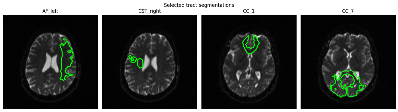
TractSeg — white matter tract segmentation
TractSeg segments 72 white matter bundles directly from CSD peaks. It can also produce tract endpoint regions and tract orientation maps (TOMs).
from kwneuro.tractseg import extract_tractseg

tracts = extract_tractseg(dwi_denoised, mask, response, output_type="tract_segmentation")
from tractseg.data.dataset_specific_utils import get_bundle_names
all_names = get_bundle_names("All")[1:]  # skip BG

tracts_arr = tracts.get_array()  # (x, y, z, 72)
print(f"TractSeg output shape: {tracts_arr.shape}")

bundle_names = [
    "AF_left",
    "CST_right",
    "CC_1", # rostrum
    "CC_7", # splenium
]
bundle_indices = [all_names.index(n) for n in bundle_names]


denoised_meanb0 = dwi_denoised.compute_mean_b0()
fig, axes = plt.subplots(1, len(bundle_indices), figsize=(14, 4))
for ax, idx, name in zip(axes, bundle_indices, bundle_names):
    bundle_data = tracts_arr[:, :, :, idx]
    best_slice_idx = bundle_data.sum(axis=(0, 1)).argmax() # Find the slice with the most segmented voxels
    ax.imshow(denoised_meanb0.get_array()[:, :, best_slice_idx].T, cmap="gray", origin="lower")
    ax.contour(tracts_arr[:, :, best_slice_idx, idx].T, colors="lime", linewidths=0.8)
    ax.set_title(name)
    ax.axis("off")
plt.suptitle("Selected tract segmentations")
plt.tight_layout()
plt.show()
TractSeg output shape: (128, 128, 60, 72)
Saving results to disk
All results can be saved to NIfTI files. save() returns a new object
backed by on-disk resources (functional style — originals are unchanged).
output_dir = Path("output")
output_dir.mkdir(exist_ok=True)

# Save DTI tensor volume
dti_saved = dti.save(output_dir / "dti.nii.gz")

# Save individual FA and MD maps
NiftiVolumeResource.save(fa_vol, output_dir / "fa.nii.gz")
NiftiVolumeResource.save(md_vol, output_dir / "md.nii.gz")

# Save NODDI (volume + directions)
noddi_saved = noddi.save(output_dir / "noddi.nii.gz")

# Save brain mask
NiftiVolumeResource.save(mask, output_dir / "brain_mask.nii.gz")

# Save the denoised DWI (volume + bval + bvec)
dwi_denoised.save(output_dir, basename="denoised_dwi")

print(f"Results saved to {output_dir.resolve()}")
Pipeline caching
Wrapping pipeline steps in a Cache context manager enables automatic
disk-based caching. Key behaviours:
First run: results are computed and saved to
cache_dir.Subsequent runs: results are loaded from disk, skipping the computation.
Scalar parameters (
int,float,str,bool) are stored as human-readable JSON and fingerprinted — changing a value invalidates that step’s cache.Input data (volumes, b-values, b-vectors, masks, response functions) are sha256-fingerprinted — if the underlying data changes, the cache is invalidated automatically.
Forced recomputation: pass
force={"step_name"}orforce=Trueto rerun a specific step or all steps regardless of cache state.
from kwneuro.cache import Cache
from kwneuro.dti import Dti
from kwneuro.noddi import Noddi

cache_dir = Path("cache")

with Cache(cache_dir) as pc:
    dti = dwi_denoised.estimate_dti(mask=mask)
    noddi = dwi_denoised.estimate_noddi(mask=mask)
    _, peaks = compute_csd_peaks(dwi_denoised, mask, response)
status = pc.status([Dti.estimate_dti, Noddi.estimate_noddi, compute_csd_peaks])
print("Cache status:")
for step, is_cached in status.items():
    print(f"  {step}: {'cached' if is_cached else 'not cached'}")
Cache status:
  Dti.estimate_dti: cached
  Noddi.estimate_noddi: cached
  compute_csd_peaks: cached
Quick look at the .params.json file saved alongside each cached step.
The sidecar has two sections:
scalars— scalar parameters stored as human-readable JSON, so you can inspect exactly what values were used to produce the cached result.hashes— sha256 fingerprints of non-scalar inputs (DWI volume, b-values, b-vectors, mask, response function, etc.). If the underlying data changes between runs, the hash changes and the cache is invalidated.
import json

print("Files in cache_dir:")
for f in sorted(cache_dir.iterdir()):
    print(f"  {f.name}")

print("\nestimate_dti.params.json:")
sidecar = json.loads((cache_dir / "estimate_dti.params.json").read_text())
print(json.dumps(sidecar, indent=2))
Files in cache_dir:
  compute_csd_peaks.params.json
  csd_peak_dirs.nii.gz
  csd_peak_values.nii.gz
  estimate_dti.nii.gz
  estimate_dti.params.json
  estimate_noddi.nii.gz
  estimate_noddi.params.json
  estimate_noddi_directions.nii.gz

estimate_dti.params.json:
{
  "hashes": {
    "dwi": "a0b14d69557b8bdba79063cd935673b8c114ffaf1c3756b87c2c930d905abc6a",
    "mask": "454054019b2fb1265fbeca5db8fb65b1701390a75d443c974e4f9896f8a71953"
  }
}