White Matter Microstructure in Persistent Psychotic-Like Experiences

A Voxelwise dMRI Study using ABCD 6.0 and kwneuro

How to read this tutorial. This document describes a real clinical study investigating white matter differences in adolescents with psychotic-like experiences. It includes illustrative Python code using the kwneuro library to demonstrate how the pipeline was implemented - from per-subject processing, to population template building, to scanner harmonisation; the reader does not need to run the code to follow the study. The voxelwise group comparison itself is left as planned analyses, and is specified in §4 as the next step of the study.

---

Abstract

Using diffusion MRI data from the Adolescent Brain Cognitive Development (ABCD) Study Release 6.0, this tutorial documents a pipeline for identifying white matter microstructural changes associated with a persistent-distressing psychotic-like experience (PLE) trajectory (n = 253), relative to a normative low-symptom trajectory (n = 253). Five microstructural metrics (FA, MD, NDI, ODI, and FWF) were estimated voxelwise, registered to a study-specific template, and harmonised across 21 scanner sites with ComBat. At the end of the tutorial, we specify the voxelwise GLM, controlling for age, sex, and household income, that will identify which metrics and regions differ between groups. The full pipeline was implemented in kwneuro, a Python library for dMRI analysis.

---

1. Introduction

Persistent, distressing psychotic-like experiences (PLEs) in adolescence are associated with elevated risk for later psychotic disorder, depression, and functional impairment[1]. Karcher et al.[2] applied latent class growth analysis to ABCD Study data and identified five PLE trajectory classes. This study contrasts Group 1 (persistent-distressing) and Group 5 (low-distressing / normative), to detect neurobiological correlates of early psychotic risk.

This tutorial demonstrates a pipeline for identifying which white matter microstructural metrics differ between adolescents on the persistent-distressing PLE trajectory and those on the normative trajectory. The voxelwise GLM (§4) tests for differences across all five metrics. This is motivated by prior work in early psychosis-spectrum experiences, which used structural MRI to show that youth with persistent distressing psychotic-like experiences (PLEs) exhibit cortical and subcortical patterns resembling those seen in adult schizophrenia spectrum and Alzheimer disease samples. Building on these findings, we sought to examine whether diffusion MRI would reveal analogous microstructural alterations, as indexed by DTI and NODDI metrics[2].

Five dMRI metrics are derived from two biophysical models.

Metric	Model	Interpretation
FA - Fractional Anisotropy	DTI	Directional coherence; non-specific
MD - Mean Diffusivity	DTI	Overall displacement; non-specific
NDI - Neurite Density Index	NODDI	Intra-neurite volume fraction
ODI - Orientation Dispersion Index	NODDI	Fibre fanning and crossing
FWF - Free Water Fraction	NODDI	Extracellular free-water compartment

This tutorial walks through the full processing pipeline - from raw DWI through scanner harmonisation - preparing the metrics and covariates that feed into the voxelwise GLM specified in §4, which is outside the scope of this tutorial.

---

2. Study Cohort

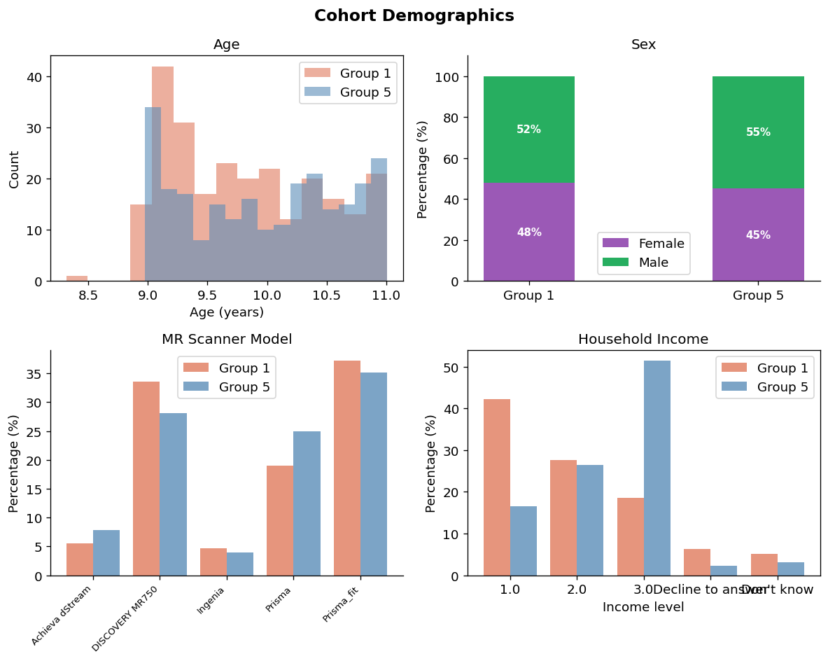
Participants were drawn from the ABCD 6.0 baseline assessment (age 9–11 years).

	Group 1 — Persistent Distressing	Group 5 — Low Distressing
N	253	253
Age	9.80 ± 0.62 years	9.98 ± 0.65 years
Female	48%	45%

Statistical models include age, sex, and household income (3-level ordinal) as covariates, selected to isolate group-related microstructural differences (§1) from known confounds of white matter development. Scanner model is treated as a batch variable and addressed via ComBat harmonisation before statistical testing.

Cohort Demographics

---

3. Analysis Pipeline

The pipeline proceeds in seven stages: (1) DWI denoising, (2) brain extraction, (3) microstructure estimation, (4) study-specific template construction, (5) subject-to-template registration, (6) ComBat harmonisation, and (7) voxelwise GLM. All stages are implemented in kwneuro, which provides transparent disk-based caching so that any step can be rerun in isolation after a parameter change.

3.1 Preprocessing and Microstructure Estimation

Denoising (Patch2Self)[3], brain extraction (HD-BET)[4], and microstructure estimation (DTI + NODDI)[5][6] are run per subject. The Cache context manager handles checkpointing so the batch loop is safely restartable.

# Illustrative — requires access to raw DWI data
from kwneuro.cache import Cache
from kwneuro.masks import brain_extract_dwi_batch


def load_denoised_dwi(sid):
    stem = str(OUT_ROOT / sid / "dwi_denoised")
    return Dwi(
        NiftiVolumeResource(stem + ".nii.gz"),
        FslBvalResource(stem + ".bval"),
        FslBvecResource(stem + ".bvec"),
    )


# --- Denoising + brain extraction ---
cases = []
for sid in participants["participant_id"]:
    raw_dir = PROJECT_ROOT / "raw_data" / sid / "dwi"
    dwi = Dwi(
        NiftiVolumeResource(raw_dir / f"{sid}_dwi.nii.gz"),
        FslBvalResource(raw_dir / f"{sid}.bval"),
        FslBvecResource(raw_dir / f"{sid}.bvec"),
    )
    with Cache(cache_dir=OUT_ROOT / sid / "cache"):
        dwi_denoised = dwi.denoise()
    dwi_denoised.save(OUT_ROOT / sid, stem="dwi_denoised")
    cases.append((dwi_denoised, OUT_ROOT / sid / "brain_mask.nii.gz"))

brain_extract_dwi_batch(cases)  # single GPU pass over all 506 subjects

# --- DTI + NODDI per subject ---
for sid in participants["participant_id"]:
    dwi_denoised = load_denoised_dwi(sid)
    brain_mask = NiftiVolumeResource(OUT_ROOT / sid / "brain_mask.nii.gz")

    with Cache(cache_dir=OUT_ROOT / sid / "cache"):
        dti = dwi_denoised.estimate_dti(brain_mask)
        fa, md = dti.get_fa_md()
        noddi = dwi_denoised.estimate_noddi(brain_mask, dpar=1.7e-3)

    for name, arr in zip(
        ["fa", "md", "ndi", "odi", "fwf"],
        [fa, md, noddi.ndi, noddi.odi, noddi.fwf],
    ):
        NiftiVolumeResource.save(arr, OUT_ROOT / sid / f"{name}.nii.gz")

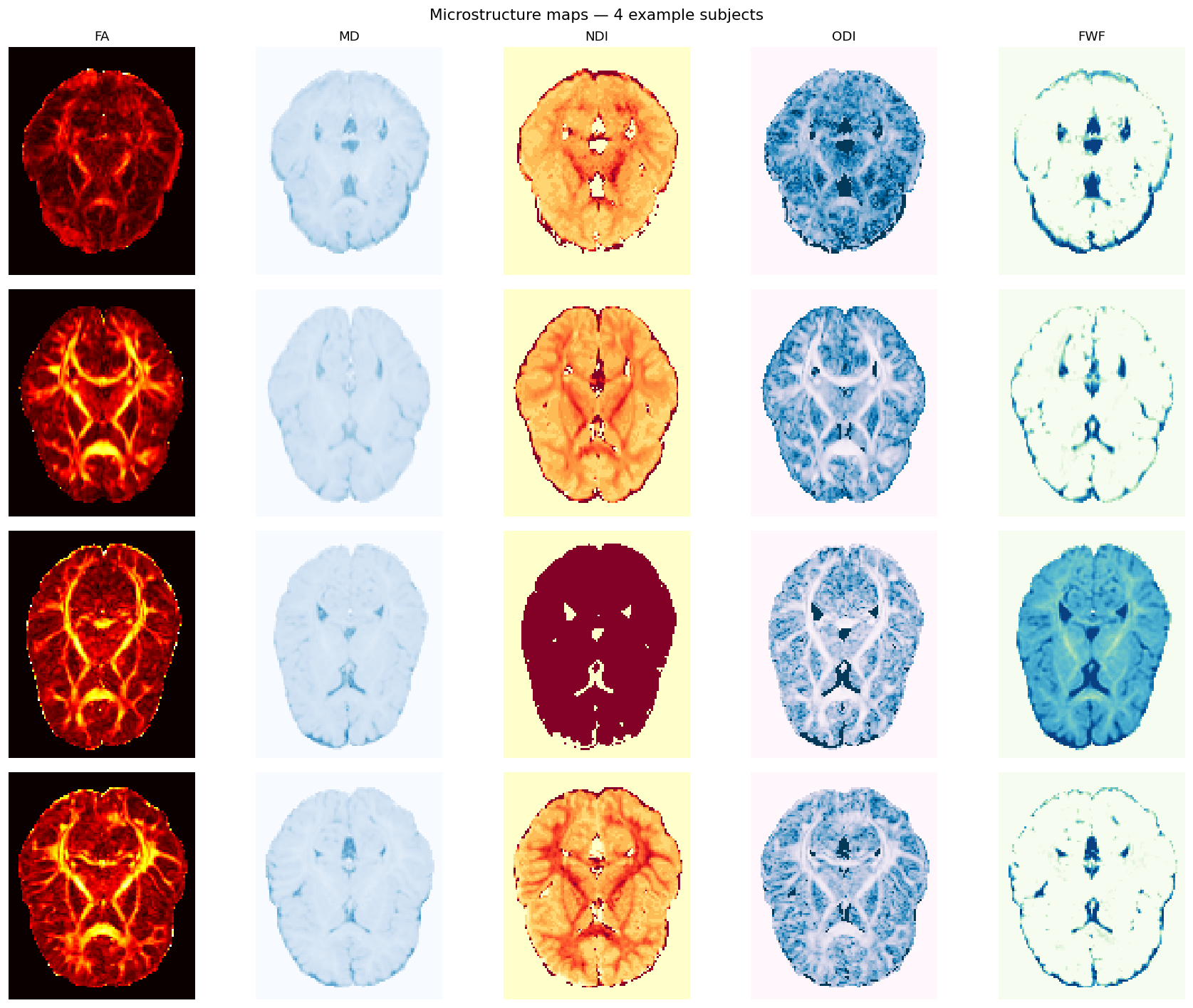
The figure below shows the five metric maps for four representative subjects — two from each group — all at the same axial slice.

3.2 Study-Specific Template Construction

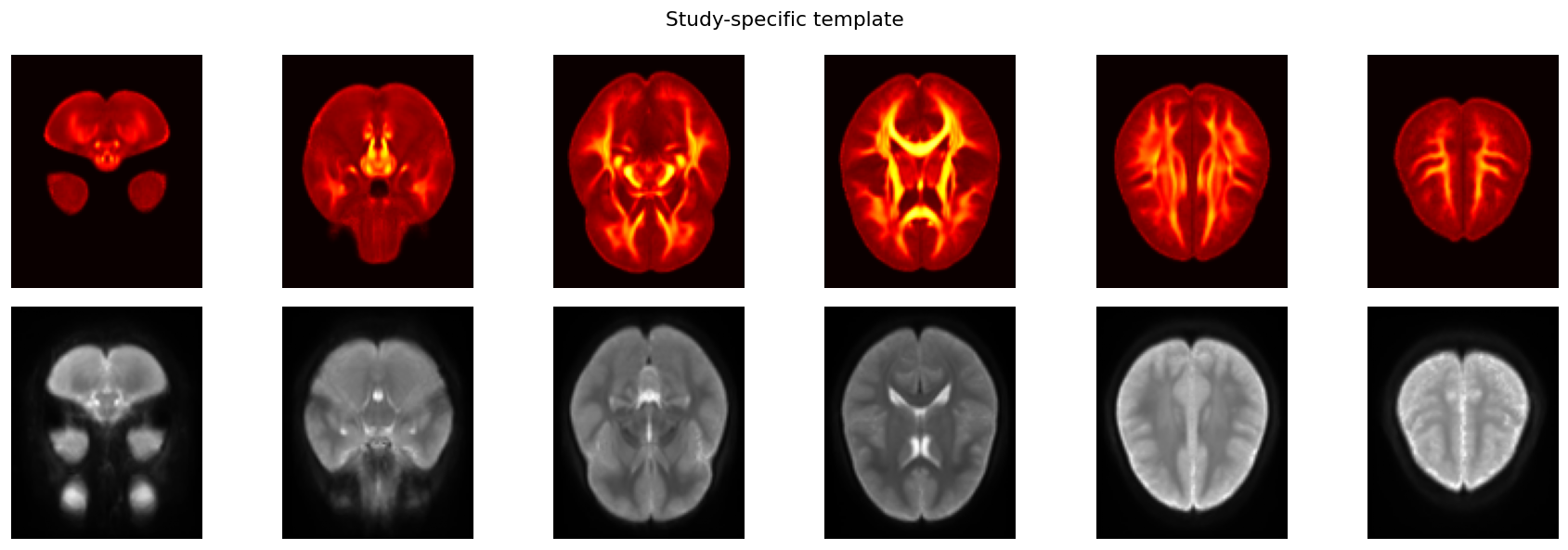
A balanced subset of 25 subjects per group (50 total) was selected with a fixed random seed to ensure neither group dominates the template geometry. The template is built jointly from FA and mean b=0 using iterative groupwise registration (ANTs)[7], capturing both white matter structure and cortical boundaries.

# Illustrative — requires per-subject metric maps
from kwneuro.build_template import build_multi_metric_template

g1_sample = g1.sample(n=25, random_state=42)
g5_sample = g5.sample(n=25, random_state=42)
template_ids = pd.concat([g1_sample, g5_sample])["participant_id"]

subject_metrics = [
    {
        "fa": NiftiVolumeResource(OUT_ROOT / sid / "fa.nii.gz"),
        "mean_b0": load_denoised_dwi(sid).compute_mean_b0(),
    }
    for sid in template_ids
]

templates = build_multi_metric_template(subject_metrics, iterations=12)
NiftiVolumeResource.save(templates["fa"], OUT_ROOT / "template" / "template_fa.nii.gz")
NiftiVolumeResource.save(
    templates["mean_b0"], OUT_ROOT / "template" / "template_mean_b0.nii.gz"
)

Study-specific template: FA (top row) and mean b=0 (bottom row) across six axial slices.

3.3 Registration to Template Space

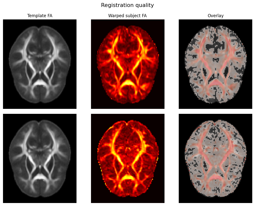
All five metric maps for each subject are warped to template space. The deformation is estimated jointly from subject FA and mean b=0 (multi-metric SyN; mutual-information cost), then applied to the remaining metrics. A per-subject white matter mask from Atropos tissue segmentation on the FA map constrains the registration optimiser to white matter.

# Illustrative — requires per-subject metric maps and template
from kwneuro.reg import register_volumes
from kwneuro.seg import segment_tissue_atropos

template_fa = NiftiVolumeResource(TEMPLATE_FA)
template_mean_b0 = NiftiVolumeResource(TEMPLATE_MEAN_B0)

for sid in participants["participant_id"]:
    fa = NiftiVolumeResource(OUT_ROOT / sid / "fa.nii.gz")
    brain_mask = NiftiVolumeResource(OUT_ROOT / sid / "brain_mask.nii.gz")

    tissue = segment_tissue_atropos(fa, brain_mask, n_classes=3)
    NiftiVolumeResource.save(tissue["wm"], OUT_ROOT / sid / "wm_mask.nii.gz")

    warped_fa, transform = register_volumes(
        fixed=[template_fa, template_mean_b0],
        moving=[fa, load_denoised_dwi(sid).compute_mean_b0()],
        type_of_transform="SyN",
        moving_mask=tissue["wm"],
    )
    NiftiVolumeResource.save(warped_fa, OUT_ROOT / sid / "fa_warped.nii.gz")
    transform.save(OUT_ROOT / sid / "transforms")

    for metric in ["md", "ndi", "odi", "fwf"]:
        warped = transform.apply(
            template_fa,
            NiftiVolumeResource(OUT_ROOT / sid / f"{metric}.nii.gz"),
        )
        NiftiVolumeResource.save(warped, OUT_ROOT / sid / f"{metric}_warped.nii.gz")

Registration quality: template FA, warped subject FA, and overlay for two example subjects.

3.4 Group White Matter Mask

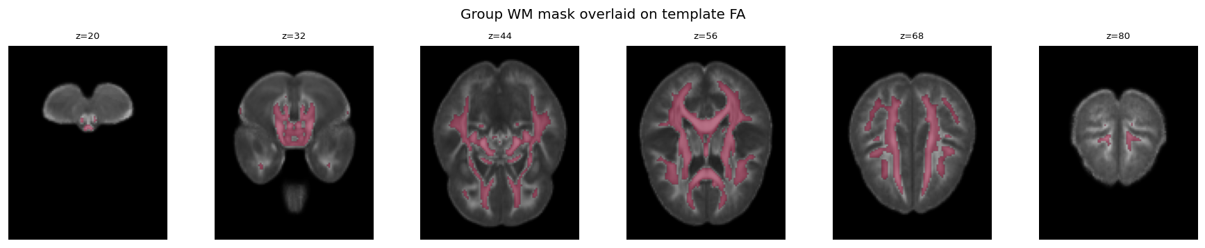
Each subject’s Atropos WM mask is warped to template space using the saved transforms. Averaging across all 506 subjects produces a voxelwise coverage fraction; voxels covered by ≥50% of subjects form the final group analysis mask used as the search volume for ComBat and the voxelwise GLM.

3.5 Scanner Harmonisation

ComBat[8][9] is applied independently per metric, removing site-specific additive and multiplicative effects while preserving variance attributable to age, sex, income, and group. §4 specifies the voxelwise GLM used to test for group differences in the harmonised metric maps.

# Illustrative — requires warped metric volumes in template space
from kwneuro.harmonize import harmonize_volumes
from kwneuro.io import NiftiVolumeResource
import nibabel as nib
import pickle

GROUP_MASK = OUT_ROOT / "template" / "group_brain_mask.nii.gz"
METRICS = ["fa", "md", "ndi", "odi", "fwf"]

# Subjects with income codes 777 (decline to answer) or 999 (don't know)
# are excluded — they cannot be used as a numeric covariate.
harm_participants = participants[~participants["income"].isin([777, 999])].reset_index(
    drop=True
)

covars = pd.DataFrame(
    {
        "scanner": harm_participants["scanner"],
        "age": harm_participants["age"],
        "income": harm_participants["income"],
        "sex_bin": (harm_participants["sex"] == "F").astype(int),
        "group": harm_participants["group"],
    }
)

brain_mask = NiftiVolumeResource(GROUP_MASK)

(OUT_ROOT / "stats").mkdir(exist_ok=True)

for metric in METRICS:
    volumes = [
        NiftiVolumeResource(OUT_ROOT / sid / f"{metric}_warped.nii.gz")
        for sid in harm_participants["participant_id"]
    ]
    harmonized, estimates = harmonize_volumes(
        volumes,
        covars,
        batch_col="scanner",
        mask=brain_mask,
        continuous_cols=["age", "income", "group"],
        categorical_cols=["sex_bin"],
    )
    for sid, harm_vol in zip(harm_participants["participant_id"], harmonized):
        nib.save(
            nib.Nifti1Image(harm_vol.get_array(), harm_vol.get_affine()),
            str(OUT_ROOT / sid / f"{metric}_warped_harmonized.nii.gz"),
        )
    with open(OUT_ROOT / "stats" / f"combat_estimates_{metric}.pkl", "wb") as f:
        pickle.dump(estimates, f)

Each dot below is one subject; horizontal bars are site medians. Sites are sorted left-to-right by their pre-harmonisation grand mean FA, so any inter-site offset is immediately visible on the left panel and should collapse on the right.

---

4. Results and Discussion

The pipeline above produces harmonised, template-space maps of FA, MD, NDI, ODI, and FWF for all 506 subjects. As shown in §3.5, ComBat harmonisation removes the site-level offsets visible in the raw metric distributions, confirming that scanner effects are adequately controlled before any group-level comparison.

Planned statistical analysis. Group differences can be identified by testing all five metrics voxelwise within the white matter mask (§3.4):

\[\text{metric} \sim \beta_0 + \beta_1 \cdot \text{group} + \beta_2 \cdot \text{age} + \beta_3 \cdot \text{sex} + \beta_4 \cdot \text{income}\]

at each WM voxel, with FDR correction (\(q < 0.05\)). Positive \(t\)-values on \(\beta_1\) indicate higher metric in Group 1 (persistent-distressing); negative values indicate lower metric. As motivated in §1, this test can be conducted across all five metrics and the full white matter mask to examine whether diffusion MRI reveals microstructural alterations analogous to the cortical and subcortical patterns previously reported with structural MRI.

---

References

---

[1]

Karcher, Nicole R., et al. (2022). Persistent and distressing psychotic-like experiences using adolescent brain cognitive development study data. Molecular psychiatry 27(3), 1490-1501.

[2] (1,2)

Karcher, N.R. et al. (2023). Trajectories of psychotic-like experiences and associations with outcomes in the ABCD Study. JAMA Psychiatry.

[3]

Fadnavis, S. et al. (2020). Patch2Self: Denoising diffusion MRI with self-supervised learning. NeurIPS, 33.

[4]

Isensee, F. et al. (2019). Automated brain extraction of multi-sequence MRI using artificial neural networks. Human Brain Mapping, 40(17), 4952–4964.

[5]

Zhang, H. et al. (2012). NODDI: Practical in vivo neurite orientation dispersion and density imaging of the human brain. NeuroImage, 61(4), 1000–1016.

[6]

Daducci, A. et al. (2015). AMICO: Accelerated microstructure imaging via convex optimization. NeuroImage, 105, 32–44.

[7]

Avants, B.B. et al. (2008). Symmetric diffeomorphic image registration with cross-correlation. Medical Image Analysis, 12(1), 26–41.

[8]

Johnson, W.E., Li, C., & Rabinovic, A. (2007). Adjusting batch effects in microarray expression data using empirical Bayes methods. Biostatistics, 8(1), 118–127.

[9]

Fortin, J.P. et al. (2017). Harmonization of multi-site diffusion tensor imaging data. NeuroImage, 161, 149–170.